1
2
3
4
5
6
7
8
9
10
11
12
13
14
15
16
17
18
19
20
21
22
23
24
25
26
27
28
29
30
31
32
33
34
35
36
37
38
39
40
41
42
43
44
45
46
47
48
49
50
51
52
53
54
55
56
57
58
59
60
61
62
63
64
65
66
67
68
69
70
71
72
73
74
75
76
77
78
79
80
81
82
83
84
85
86
87
88
89
90
91
92
93
94
95
96
97
98
|
"""
作者:冯振华
学号:202221140015
版本:V4.1
日期:2023年05月20日
项目:Monte Carlo methods for Overcoming critical slowing down
"""
import numpy as np
import matplotlib.pyplot as plt
def initialize_spins(N):
"""
Initializes the spin lattice with random spins of -1 or +1
"""
return np.random.choice([-1, 1], size=(N, N))
def bond_probability(beta):
"""
Calculates probability of forming a bond between two neighboring spins
"""
return 1 - np.exp(-2*beta)
def update_spins(spins, beta):
"""
a single update of the spins using the Wolff algorithm
"""
N = spins.shape[0]
visited = np.zeros((N, N), dtype=bool)
seed = (np.random.randint(N), np.random.randint(N))
cluster_spins = [seed]
cluster_perimeter = [(seed[0], (seed[1]+1)%N), (seed[0], (seed[1]-1)%N),
((seed[0]+1)%N, seed[1]), ((seed[0]-1)%N, seed[1])]
while len(cluster_perimeter) > 0:
i, j = cluster_perimeter.pop()
if not visited[i,j] and np.random.random() < bond_probability(beta):
cluster_spins.append((i, j))
visited[i, j] = True
cluster_perimeter += [(i, (j+1)%N), (i, (j-1)%N),
((i+1)%N, j), ((i-1)%N, j)]
spins[tuple(zip(*cluster_spins))] *= -1
return spins
def calculate_energy(spins,J):
"""
Calculates the energy of the spin configuration
"""
N = spins.shape[0]
energy = 0
for i in range(N):
for j in range(N):
spin = spins[i, j]
neighbors = spins[(i+1)%N, j] + spins[i, (j+1)%N] + spins[(i-1)%N, j] + spins[i, (j-1)%N]
energy += 2*J*spin * neighbors
return energy
def run_simulation(N=20, J=-1,beta=1.0, num_steps=2000, num_measurements=100):
"""
Performs a full simulation of the Wolff algorithm on the spin lattice
"""
spins = initialize_spins(N)
energies = []
mags = []
for step in range(num_steps):
spins = update_spins(spins, beta)
if step % (num_steps // num_measurements) == 0:
energy = calculate_energy(spins,J)
mag = np.sum(spins)
energies.append(energy)
mags.append(mag)
return energies, mags
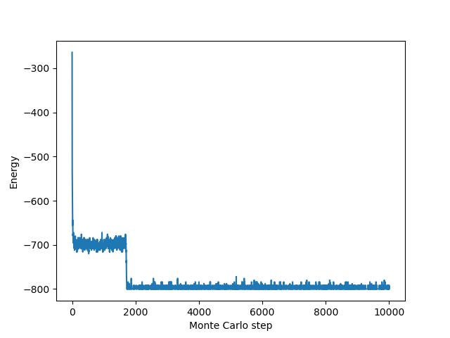
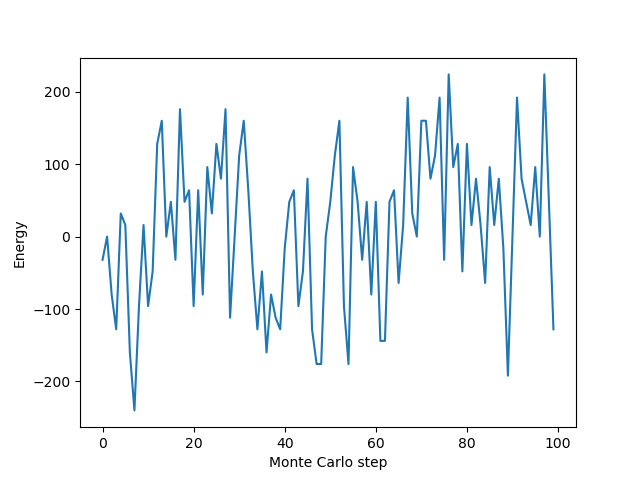
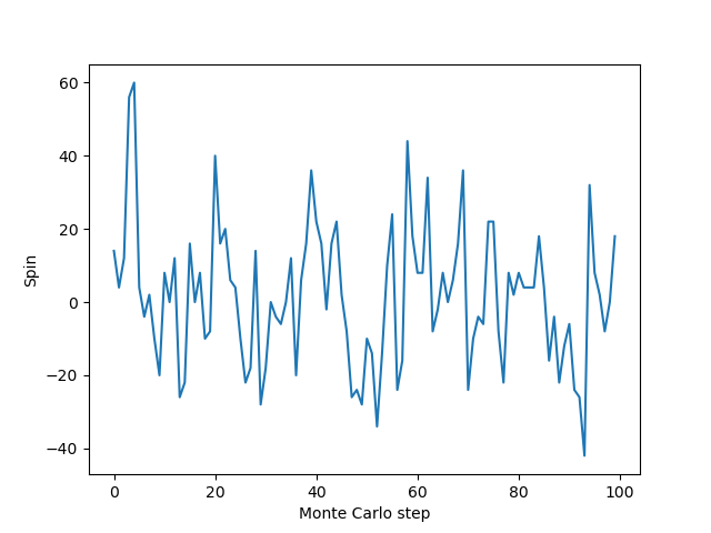
energies, mags = run_simulation(N=20,J=-1,beta=1.0, num_steps=100000, num_measurements=100)
E = np.mean(energies)
print(f"Average energy: {E:.4f}")
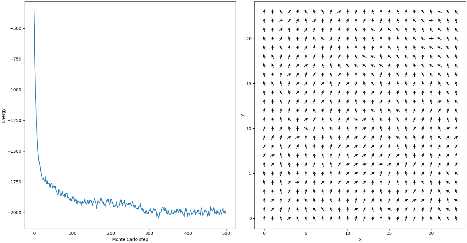
plt.plot(energies)
plt.xlabel("Monte Carlo step")
plt.ylabel("Energy")
plt.show()
plt.plot(mags)
plt.xlabel("Monte Carlo step")
plt.ylabel("Spin")
plt.show()
"""
To run the simulation, simply the `run_simulation` function with the desired parameters, such as `energies, mags = run_simulation(N=30,=1.0, num_steps=100000, num_measurements=100)`. This will simulate 100,000 Wolff updates on a 30x30 lattice at a temperature of 1. and take measurements of the energy and magnetization every 1,000 steps. The output is two arrays, `energies` and `mags`, that record the energy and magnetization at each measurement step. These arrays can be used to averages and variances to analyze the system properties.
"""
|